Learn
Build Your First Virtual Economy#
In this tutorial, you will create a virtual economy populated by workers, firms, and banks, run it for 1,000 time steps, and watch macroeconomic patterns emerge from individual agent decisions. Then you will add technological change with three lines of code and see how the economy transforms.
What you will need:
- Python 3.11 or later
- BAM Engine installed:
pip install bamengine - Matplotlib for plotting:
pip install matplotlib
Setting Up the Economy#
Every simulation starts with Simulation.init(), which creates the
agents and sets up the economy:
import bamengine as bam

sim = bam.Simulation.init(
    n_firms=100,        # 100 companies that produce goods
    n_households=500,   # 500 people who work and consume
    n_banks=10,         # 10 banks that provide credit
    seed=42,            # Fixed seed for reproducible results
)
Here is what each argument does:
n_firms: The number of firms in the economy. Each firm sets prices, hires workers, borrows from banks, produces goods, and sells them to consumers.n_households: The number of households. Each household seeks employment, earns wages, and spends money on goods.n_banks: The number of banks. Banks receive deposits, evaluate loan applications, and provide credit to firms.seed: A random seed for reproducibility. Using the same seed always produces the same simulation results. Change the seed to see different realizations of the same economy.
Behind the scenes, init() assigns initial conditions to every agent
(starting prices, wages, inventories, cash balances) and builds the event
pipeline, the sequence of economic actions that happen each period.
Running the Simulation#
Now let’s run the economy for 1,000 time steps:
results = sim.run(
    n_periods=1000,     # Simulate 1000 economic cycles
)n_periods: How many time steps to simulate. Each period represents one complete economic cycle: firms plan production, hire workers in the labor market, borrow from banks in the credit market, produce goods, sell in the goods market, pay dividends, and update their books.
sim.run() automatically collects per-agent data at every time step
and returns a SimulationResults object. You can access the data using
bracket notation (results["Role.variable"]) or attribute-style access
(results.Role.variable).
In the plots below, we skip the first 200 periods (the “burn-in”). Agent-based models start from artificial initial conditions (all firms identical, no one employed, no loans outstanding), so the first few hundred periods are dominated by the economy organizing itself rather than exhibiting natural dynamics. Skipping this transient phase lets us focus on the settled behavior.
Unemployment#
Unemployment is computed from the per-household employment status:
import matplotlib.pyplot as plt
import numpy as np
from bamengine import ops

burn_in = 200  # Skip initial transient before the economy settles

# Get employment status: shape (n_periods, n_households)
employed = results.Worker.employed

# Unemployment rate = fraction of workers without a job
unemployment = 1 - np.mean(employed.astype(float), axis=1)

plt.figure(figsize=(10, 4))
plt.plot(unemployment[burn_in:], linewidth=0.8)
plt.xlabel("Period")
plt.ylabel("Unemployment Rate")
plt.title("Unemployment Rate Over Time")
plt.tight_layout()
plt.show()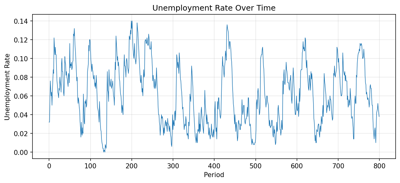
results.Worker.employed returns a 2D NumPy array with shape
(n_periods, n_households), where each value is True if the household
has a job and False otherwise. Averaging across households (axis=1)
gives the employment rate; subtracting from 1 gives the unemployment
rate.
Notice the oscillations: these are business cycles, and they were not programmed. There is no “recession function” or “boom equation” in the code. Each firm independently decides how many workers to hire based on its own sales, and each household independently searches for jobs. When many firms cut production at once, unemployment rises; when they expand, it falls. The entire pattern emerges from the bottom up, from thousands of simple, local decisions interacting through markets.
Inflation#
Inflation measures how the average market price changes from period to period:
inflation = results["Economy.inflation"]

plt.figure(figsize=(10, 4))
plt.plot(inflation[burn_in:], linewidth=0.8, color="tab:orange")
plt.xlabel("Period")
plt.ylabel("Inflation Rate")
plt.title("Inflation Rate Over Time")
plt.tight_layout()
plt.show()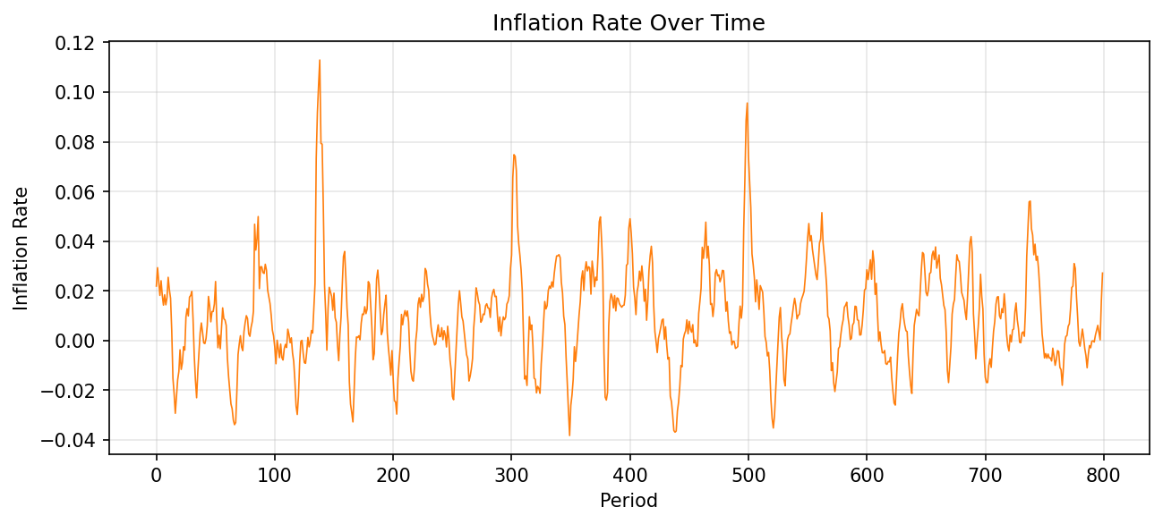
Again, no one told the economy what inflation rate to produce. Each firm independently adjusts its price based on a simple rule: if it sold out, raise the price; if it had leftover inventory, lower it. The aggregate inflation pattern is a collective outcome of thousands of individual pricing decisions, none of which have any knowledge of the “big picture.”
GDP#
GDP (Gross Domestic Product) is the total production of all firms. Since we collected per-firm production data, we can compute it:
# Get production data: shape (n_periods, n_firms)
production = results.Producer.production

# GDP = sum of all firms' production each period
gdp = ops.sum(production, axis=1)

plt.figure(figsize=(10, 4))
plt.plot(gdp[burn_in:], linewidth=0.8, color="tab:green")
plt.xlabel("Period")
plt.ylabel("Total Production (GDP)")
plt.title("Real GDP Over Time")
plt.tight_layout()
plt.show()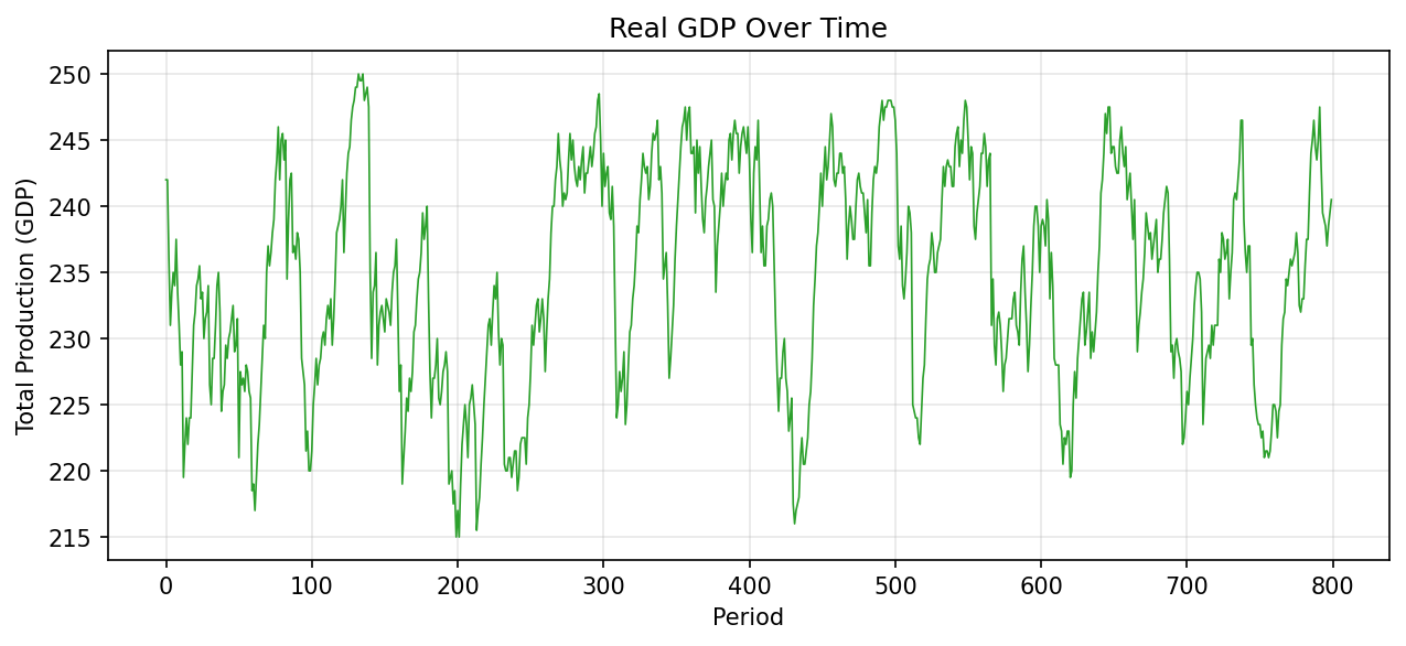
results.Producer.production returns a 2D NumPy array with shape
(n_periods, n_firms). Summing across firms (axis=1) gives total GDP
each period.
GDP is not a variable in the model. No equation computes it. It is simply the sum of what every firm happened to produce, and that depends on how many workers each firm managed to hire, how much credit it could secure, and what price it set. The macroeconomic output is an emergent property of microeconomic interactions.
In the baseline model (without R&D), GDP fluctuates around a relatively stable level. There is no long-run growth because firms cannot innovate; they produce with fixed technology.
Wages and Productivity#
Let’s compare the average real wage to average productivity:
# Average price each period (for converting nominal to real)
avg_price = results["Economy.avg_price"]

# Worker wages
wages = results.Worker.wage

# Average wage among employed workers
wages_employed = ops.where(employed, wages, 0.0)
employed_float = employed.astype(float)
avg_wage = ops.divide(
    ops.sum(wages_employed, axis=1),
    ops.sum(employed_float, axis=1),
)
real_wage = ops.divide(avg_wage, avg_price)

# Production-weighted average productivity
productivity = results.Producer.labor_productivity
weighted_prod = ops.sum(ops.multiply(productivity, production), axis=1)
avg_productivity = ops.divide(weighted_prod, gdp)

plt.figure(figsize=(10, 4))
plt.plot(real_wage[burn_in:], linewidth=0.8, label="Real Wage")
plt.plot(avg_productivity[burn_in:], linewidth=0.8, label="Avg Productivity")
plt.xlabel("Period")
plt.ylabel("Value")
plt.title("Real Wage vs. Productivity")
plt.legend()
plt.tight_layout()
plt.show()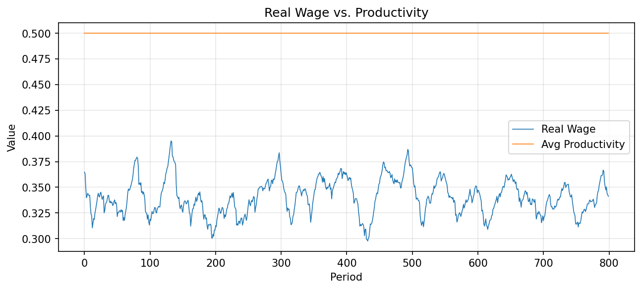
In the baseline model, real wages and productivity track each other closely. Without innovation, both remain relatively flat over time.
Adding Innovation: The R&D Extension#
What happens when firms can invest in research and development? BAM Engine’s extension system lets you find out with three extra lines:
from extensions.rnd import RND

sim = bam.Simulation.init(
    n_firms=100,
    n_households=500,
    n_banks=10,
    seed=42,
)
sim.use(RND)
results = sim.run(n_periods=1000)
from extensions.rnd import RND: imports the R&D extension bundle, which contains new roles (R&D intensity for each firm), new events (firms invest in R&D, productivity grows), and configuration parameters.sim.use(RND): activates the extension. This adds the R&D components to the simulation and inserts the new events into the pipeline at the right points.
Now let’s see what changed:
production_rnd = results.Producer.production
gdp_rnd = ops.sum(production_rnd, axis=1)

plt.figure(figsize=(10, 4))
plt.plot(gdp_rnd[burn_in:], linewidth=0.8, color="tab:green")
plt.xlabel("Period")
plt.ylabel("Total Production (GDP)")
plt.title("Real GDP with R&D Extension")
plt.tight_layout()
plt.show()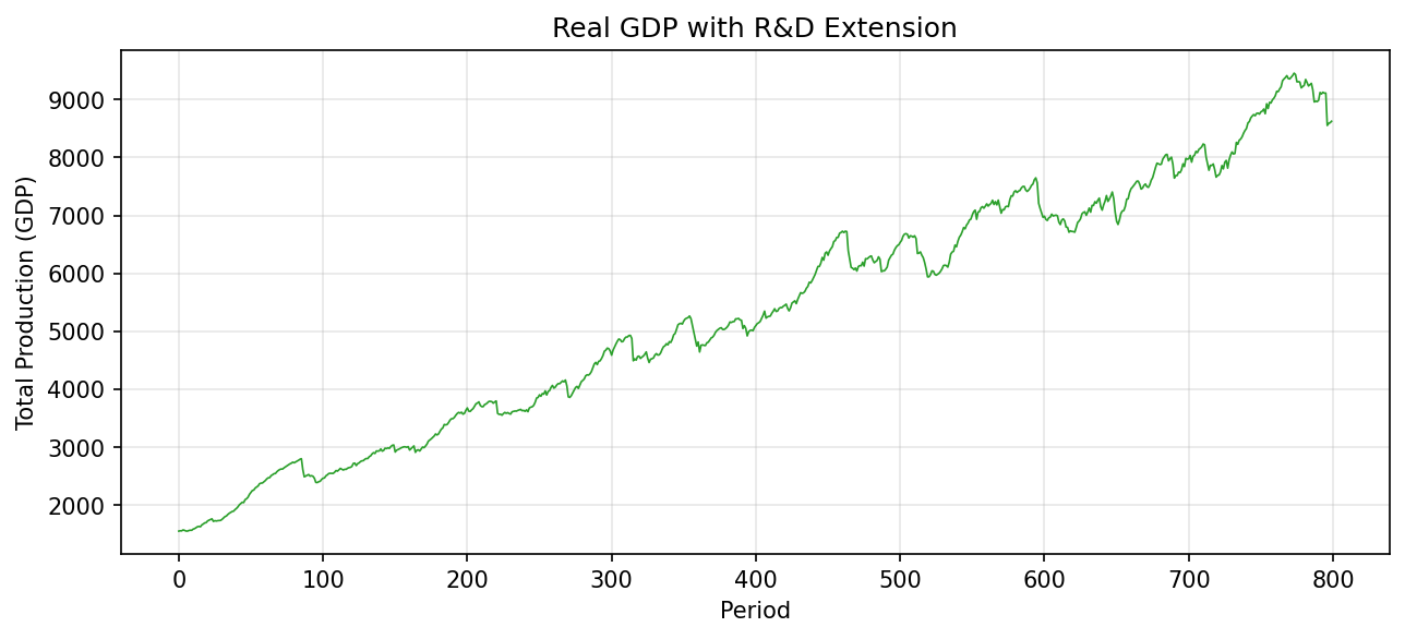
GDP now shows a clear growth trend. Firms invest a fraction of their profits in R&D, which probabilistically increases their labor productivity. Higher productivity means more output per worker, which accumulates into economy-wide growth.
Notice that the business cycle dynamics are still present: even with growth, the economy oscillates around the trend. Recessions and expansions continue to emerge from agent interactions, but now they ride on top of a rising trajectory rather than a flat baseline.
avg_price_rnd = results["Economy.avg_price"]
wages_rnd = results.Worker.wage
employed_rnd = results.Worker.employed
employed_float_rnd = employed_rnd.astype(float)
wages_employed_rnd = ops.where(employed_rnd, wages_rnd, 0.0)
avg_wage_rnd = ops.divide(
    ops.sum(wages_employed_rnd, axis=1),
    ops.sum(employed_float_rnd, axis=1),
)
real_wage_rnd = ops.divide(avg_wage_rnd, avg_price_rnd)

productivity_rnd = results.Producer.labor_productivity
weighted_prod_rnd = ops.sum(
    ops.multiply(productivity_rnd, production_rnd), axis=1
)
avg_productivity_rnd = ops.divide(weighted_prod_rnd, gdp_rnd)

plt.figure(figsize=(10, 4))
plt.plot(real_wage_rnd[burn_in:], linewidth=0.8, label="Real Wage")
plt.plot(avg_productivity_rnd[burn_in:], linewidth=0.8, label="Avg Productivity")
plt.xlabel("Period")
plt.ylabel("Value")
plt.title("Real Wage vs. Productivity (with R&D)")
plt.legend()
plt.tight_layout()
plt.show()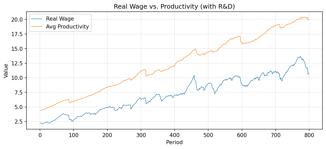
With R&D, productivity grows faster than wages, a well-known feature of innovation-driven economies. The gap between productivity and real wages reflects that not all productivity gains are immediately passed through to workers.
With three extra lines of code (import, activate, run), you have added technological change to the economy.
What’s Next?#
You have built a virtual economy, observed business cycles, and added innovation. Here is where to go from here:
- Documentation: Full user guide covering configuration, custom roles and events, pipeline customization, and the operations module
- Examples: 16 runnable examples from basic usage to advanced customization
- Gallery: More simulation output from all scenarios
- Validation Dashboard: See how simulation results compare to the published reference